Methods

    Automatic systems for measuring atmospheric CO₂ mixing ratios at high absolute accuracy and precision developed by Bakwin et al.(Balwin et al., 1995, 1998; Zhao et al., 1997)  are used. The systems use commercially available instrumentation and high-quality CO₂ mixing ratio standard gases. This methodology was deployed on the WITN TV tower (600m tall) in North Carolina and functioned for 7 years, and has operated on the WLEF Public Television tower (447m tall) in northern Wisconsin since 1994. This method has been proven capable of approximately 0.2 ppm precision and absolute accuracy. Continuous data is acquired except during periodic automated calibration. The WLEF and WITN measurements have been extensively compared to NOAA CMDL’s flask CO₂ observations (Bakwin et al., 1995, 1998; Zhao et al., 1997).

The apparatus for the measurements

 For more details for parts, click <Here>

Steps for measurements

1 The sample air is dried to reduce the water vapor interference and dilution effects.

2 Analysis for CO₂ mole fraction is carried out by IR absorption spectroscopy using a Li-Cor model 820 analyzer.

3 Calibration using high-quality standard gases is carried out every 2 hours, as described below.

Example of calibration procedure

   Calibration is a key step in the measurements, which is dependent upon high-quality calibration gases (Bakwin et al, 1995, 1998 ; Zhao et al., 1997). To assure the stability of long-term high-precision measurements of CO2 mixing ratio and cross-calibration of field sites, the standard gases have to be provided via a calibration lab, such as the one set up at Penn State. This calibration system uses four NOAA CMDL primary standard calibration tanks to calibrate the four calibration tanks to be used at each instrumented surface layer tower.  Calibration activities were closely coordinated with NOAA CMDL to assure high data quality. 
 
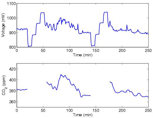
    An approximately four-hour time series of raw voltages is shown in the upper panel of the above figure.  Every two hours, a calibration sequence begins in which we sample each of four calibration tanks containing dry air with precisely known quantities of CO2 at about 330, 360, 390, and 420 ppm.  Each calibration sequence lasts eight min for each gas, for a total of 32 min.  Frequent sampling of the calibration gases is necessary in order to account for the changing response of the CO2 gas analyzer (primarily) with temperature and pressure.  Next a second-order polynomial describing the change in voltage with CO2 concentration is determined for each calibration cycle.  For example, the polynomial for the first calibration cycle in the above figure is [CO2] = 29.11 + 0.35V + 0.000037V^2, where the CO2 concentration is in ppm and the voltage is in mV.  The polynomial for the second calibration cycle is [CO2] = 39.25 + 0.32V + 0.000050V^2.  We use the average of the coefficients of these two polynomials to determine the CO2 concentration from the voltage between the two calibration cycles.  The resulting CO2 concentration during the time in which atmospheric air was sampled is shown in the lower panel of the above figure.  

    To assess the accuracy of the measurements, a set of three gases with known CO2 concentrations was tested at each site.  A limited amount of flask sampling could also be adopted at a subset of flux sites if it is proven to be desirable.  Another possiblity is leaving an "archive tank" at each site to test for long term stability of the measurements despite necessary calibration tank replacement (about four months of continuous operation.)